Get the geography
I searched, and then found, the 2022 Congressional districts shapefile
I downloaded the file, and unzipped it into a folder.
You may use a different folder
```{r}
library(tidyverse)
library(sf)
# https://catalog.data.gov/dataset/2022-cartographic-boundary-file-shp-118th-congressional-districts-for-united-states-1-20000000
wd <- getwd()
# You could easily do this a different way!
folder <- paste0(wd,"/","posts/RWithoutStatistics/")
datafolder <- paste0(folder,"/CD2022/")
# Then, read the file
CD2022 <- read_sf(paste0(datafolder,"cb_2022_us_cd118_20m.shp"))
#Check it out on the map
CD2022 %>%
ggplot() +
geom_sf(
color = "#00ff00",
linewidth = 1
)
## Ok, this worked great.
# it maps HI and AK including the Aleutians.
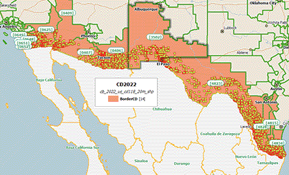
## Let's focus on the US-Mexico border.
```Border areas
I’m sure there’s a way in RStats to develop the US-Mexico border districts, but for me, I have my Scan/US subscription at hand (Scan/US web page). (disclaimer: I am a Scan/US employee, all opinions expressed here are my own) I load the shapefile into Scan/US, use my mouse to draw a polygon around the congressional districts on the border to create a grouping, and export the GEOIDs (Geographic ID’s) for the Congressional Districts on the US-Mexico border, using Scan/US’s “Export Data” menu entry. (Border Congressional districts shown in orange below)
format the vector!
Get the district array in the right format. 🍸🙀
```{r}
# Not correct
BorderDistricts <- c (0648,0650,0651,0652,0406,0625,0407,0409,3502,4823,4834,4828,4815,0649)

# also not correct -- I thought it was in character, with elided zeroes.  Nope!
BorderDistricts <- c (648,650,651,652,406,625,407,409,3502,4823,4834,4828,4815, 649)

# Correct!  A character match will work
BorderDistricts <- c ("0648","0650","0651","0652","0406","0625","0407","0409","3502","4823","4834","4828","4815","0649")

BorderCD <- CD2022 |> filter(GEOID %in% BorderDistricts)
```
Ok now get the EPA points
This URL (below) might change, you never know, but at the moment it works:
```{r}
# Get the file https://www.epa.gov/frs/epa-frs-facilities-state-single-file-csv-download
### Referred to on this site: https://www.epa.gov/frs/geospatial-data-download-service

epa_frs <- read_csv("/Users/georgegirton/Downloads/Facilities/national_single/NATIONAL_SINGLE.CSV")
problems(epa_frs)

what <- unique(epa_frs$NAICS_CODE_DESCRIPTIONS)
what
# what |> write_file("epa_frs.txt") # Error: Expected string vector of length 1

# 'cats' is short for categories.  It has nothing to do with actual 🐈🐈🐈
outfile <- paste0(folder,"cats.txt")
for(i in 1:length(what)){
  readr::write_file(paste0(what[i],"\n"),outfile, append = TRUE)
}
```
Some filtering
Choose the fields to to keep (with dplyr’s ‘select’), filter out other countries, and distill a list of locations within 100 miles of th US Mexico border, using the criterion
US_MEXICO_BORDER_IND ==“Yes”
```{r}
keepfields <- c (REGISTRY_ID, PRIMARY_NAME, NAICS_CODE_DESCRIPTIONS, LOCATION_ADDRESS, CITY_NAME,STATE_CODE,COUNTRY_NAME,CONGRESSIONAL_DIST_NUMBER,LONGITUDE83,LATITUDE83)

OtherCountries <- c ("AFGHANISTAN","ALBANIA","ALGERIA","AMERICAN SAMOA","AUSTRALIA","BASSAS DA INDIA","BELARUS","BR","BRAZIL","BRITISH VIRGIN ISLANDS","BURKINA FASO","CANADA","CHINA","COOK ISLANDS","DOMINICAN REPUBLIC","EAST TIMOR","FRANCE","GEORGIA","GERMANY","GREAT BRITAIN (UK)","GREECE","GUADELOUPE","GUAM","HONG KONG","INDIA","ISRAEL","KIRIBATI","MALAYSIA","MAURITIUS","MEXICO","MX","NETHERLANDS","NORTHERN MARIANA ISLANDS","NORWAY","PORTUGAL","PUERTO RICO","RQ","SAINT KITTS AND NEVIS","SAIPAN","SENEGAL","SUDAN","TAIWAN","THE GAMBIA","UGANDA","UNIT","UNITED ARAB EMIRATES","UNITED KINGDOM","UNITED STATES MINOR OUTLYING ISLANDS","URUGUAY","US MINOR OUTLYING ISLANDS","UZBEKISTAN","VANUATU","VATICAN CITY STATE (HOLY SEE)","VENEZUELA","VIET NAM","VIRGIN ISLANDS (U.S.)","VQ")

reduced <- epa_frs |>
  select(REGISTRY_ID, PRIMARY_NAME,US_MEXICO_BORDER_IND,INTEREST_TYPES,NAICS_CODE_DESCRIPTIONS, LOCATION_ADDRESS, CITY_NAME,     STATE_CODE,COUNTRY_NAME,CONGRESSIONAL_DIST_NUM,LONGITUDE83,LATITUDE83)

usa_only_coords <- reduced |>
  filter(!COUNTRY_NAME %in% OtherCountries) |>
  filter(!is.na(LONGITUDE83))

## 'Yes' means within 100 km of the border
nearborder <- usa_only_coords |>
    filter(US_MEXICO_BORDER_IND =="Yes")

```
Aaaand …. mapping
```{r}
nearborder |> ggplot(aes(x=LONGITUDE83, y=LATITUDE83)) + geom_point()
# that worked great
BorderCD$centroid <- st_centroid(BorderCD$geometry)
# I got these three lines from Bing. And not Bing Crosby either. Thanks, Bing!
BorderCD$coords <- st_coordinates(BorderCD$centroid )
# The x and y coordinates can be accessed as follows:
BorderCD$x <- BorderCD$coords[,1]
BorderCD$y <- BorderCD$coords[,2]
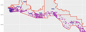
```Now, getting back to business
```{r}
    BorderCD |>  ggplot() +
  geom_sf( color = "#ff0000", linewidth = 1) +
  geom_point(data = nearborder,
    aes(x=LONGITUDE83, y=LATITUDE83),
    shape = 21, size = 1, fill = "#ff7400", color = "purple"
  ) +
  geom_text(data= BorderCD,
            aes(x=x, y=y, label=GEOID),
            color = "darkblue", fontface = "bold",
            check_overlap = FALSE)
```
Some more exploratory data exploration
```{r}
unique(nearborder$STATE_CODE)
table(nearborder$STATE_CODE)

nearborder$CD <- paste0(nearborder$STATE_CODE,nearborder$CONGRESSIONAL_DIST_NUM)
table(nearborder$CD)

nearborder <- nearborder |> filter(STATE_CODE %in% c("CA","AZ","NM","TX"))
table(nearborder$CD)
```
Welcome to the Tacos Cult of Actions!
Did you follow along successfuly? Welcome to the action cult & treat yourself to a taco! 
— all photos Copyright © 2022-2026 George D Girton all rights reserved